Concepts

Filtering and display

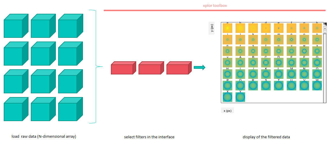
XPLOR allows users to easily visualize their multi-dimensional data. Its base principle is to apply filters on the data to select a sub-portion of it that will be displayed. In XPLOR terminology, data refers to the original data, while the displayed sub-portion is called a slice.

Steps in using XPLOR

XPLOR window

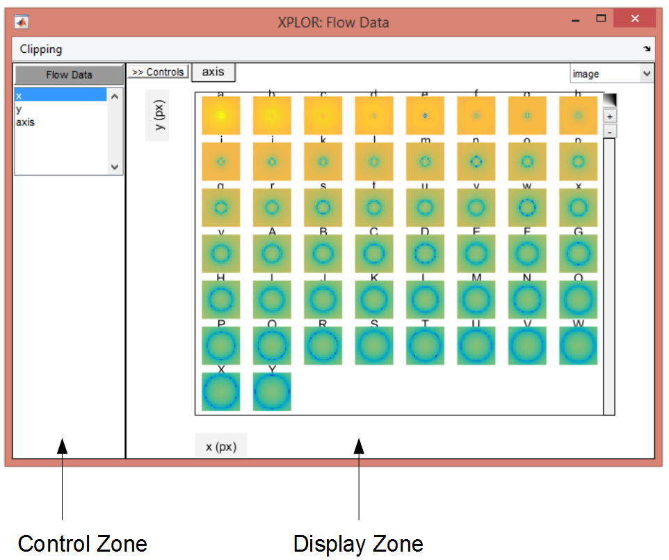
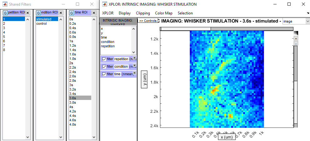
The organization of the XPLOR window reflects this principle as it is composed of a control zone on the left, where the user selects the filters to apply; and of a display zone on the right, where a number of interactions are possible such as reorganizing the layout by moving the labels’ accross axes, zooming, etc.

Screenshot of the Window with the control zone and the display zone

Labelled data

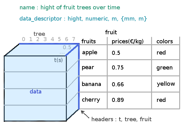
To appropriately display labels and scales, XPLOR needs to know what the data values, and what each data dimension, represents (time, space, unit, etc.). Any input data is therefore converted first to an xplr.XData object, which is a container for the N dimensional data and all the relative metadata.

Example of a Xdata instance

Filter object

Filters apply to one or several specific dimension(s) of a labelled data (i .e. of an xplr.XData object) and return a labelled data.

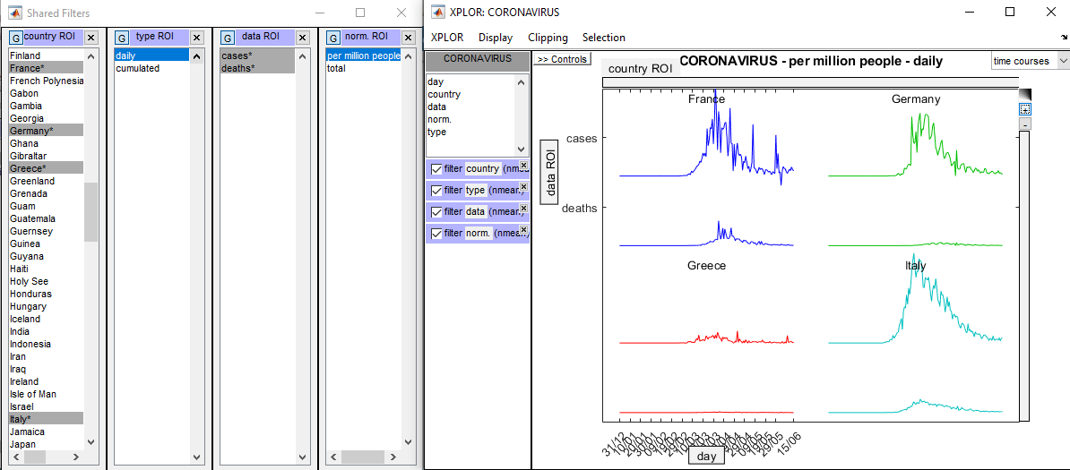
In the example below:

• the initial data has 5 dimensions: ‘day’, ‘country’, ‘type’, ‘data’ and ‘norm.’, its size is (168 x 200 x 2 x 2 x 2)
• 4 filters are applied to dimensions ‘country’ (4 countries selected), ‘type’ (1 value selected), ‘data’ (2 values) and ‘norm.’ (1 value)
• the resulting slice still has 5 dimensions: ‘day’, ‘country’, ‘type’, ‘data’ and ‘norm.’, but its size is reduced to (168 x 4 x 1 x 2 x 1); only 3 dimensions have more than one value: ‘day’, ‘country’ and ‘data’
• this slice is displayed in the display part: dimension ‘day’ is located in x and is used to form signals (it is called an internal dimension), dimension ‘data’ is dispatched vertically and dimension ‘country’ is dispatched as a 2x2 grid (they are called external dimensions).

Screenshot of the Window showing the filter applied

Zoom filters

The slice can be furthered reduced by zooming into it. It is possible to zoom in either by dragging a rectangle with the mouse left button, using the scroll wheel, or manipulating the sliders on the display side (see screenshot below). The result of zooming is called the zslice, it is again an xplr.XData object.

Slicing chain

The diagram below details the steps of applying filters and zoom filters to an original data, and shows some of XPLOR’s internal objects being involved. It follows the example of the previous screenshot:

• The original data has 5 dimensions: ‘x’, ‘y’, ‘time’, ‘condition’ and ‘repetition’
• 3 successive filters are applied respectively on dimensions ‘condition’, ‘repetition’ and ‘condition’. Each intermediary step is stored in a distinct xplr.XData object, together they form the so-called slicing chain, which is stored inside a new XPLOR object: the slicer (this object is responsible for applying filter operations each time the original data or a filter has been modified). The result of this slicing chain in the slice.
• This slice itself is the initial element of a second slicing chain handled by XPLOR’s zoom slicer object: 2 zoom filters are applied, respectively in the ‘x’ and ‘y’ dimensions. The final result is the zslice that is displayed (as in the figure above).

Synchronizing windows

The diagram below now shows the implementation of a more complex situation with two lists, a spatial display and a temporal display of the same original data.

• The lists filter the ‘condition’ and ‘repetition’ conditions for both displays.
• In the spatial display, one can either move the cross or draw spatial regions of interest to control the 2D filter applied in dimension ‘x-y’ to the data appearing in the temporal display.
• And vice-versa, in the temporal display one can either move the cross or draw temporal regions of interest that control the filter in dimension ‘time’ applied to the data shown in the spatial display.

Beneath each display are shown the filters controlling what is shown in the display (they appear in the slicing chain and zoom slicing chain already commented above), but also the filters being controlled by the lists and by the displays.

All colored elements in the diagram are filters and zoom filters. A single filter (or zoom filter) object appears at several places in the diagram. Indeed it appears both where it is controlling and where it is being controlled (and it can be controlling in several displays, as is the case for the ‘condition’ and ‘repetition’ filters; it could also be controlled in several displays though there is no such case here). In addition it also appears in a new XPLOR object that we introduce here: the bank, which keeps pointers on every existing filter and zoom filter.

Finally, red texts and arrows show an example sequence of events occuring when the user performs an action in a display: here select a new region of interest in the spatial display.